Sentiment Analysis to Improve Stock Prediction

I. Motivation

Along with the rise of machine learning, sentiment analysis has caught the attention of many researchers, the study of classifying the sentiment of text as positive and negative. Some researchers have attempted to combine sentiment analysis with stock prediction to obtain more accurate stock predictions. Combining financial news, fundamental financial company data, and historical stock data, we hope the train a classification model that predicts stock movements of popular companies accurately, and overall gives us a more comprehensive understanding of the stock market.

Stock prediction has been a popular topic for many years but most people approaches this problem by analyzing the stock performance in the past to obtain insights about market returns in the future. This approach has been proven to have many shortcomings since company’s performance is not linear and their stock data alone won’t be comprehensive enough to predict their stock movements in the future.
The objective of our research is take into account emotional states of a company combine with many quarterly fundamental data of companies to obtain a more comprehensive stock prediction model

II. Approach

1. Data Description

Our final dataset is the combination of historical stock data that reflects the pattern of stock movements, fundamental parameters that indicate the long-term financial health of a company, and the sentiment scores that symbolize the public opinions towards the given company.

Data source 1: Financial quantitative data

There are 2 sources of financial data that we use in the analysis -Daily historical stock price that we get from Yahoo Finance -The fundamental information of a company’s stocks, which has 198 features including figures such as debt, equity, book values, etc. We get this data from GuruFocus

Data source 2: Financial news

We obtained financial news data by scraping articles related to 21 popular companies that have regularly appeared on the news from 01/01/2011 to the present. Although this was supposed to give us approximately 45,000 instances of various news events, there are many days where the observed companies don’t have any news, so after dropping all of the days with no news, we were left with a sample size of approximately 25,000 instances.

In this format, wi=1 if word i is in the given piece of news. Then, we fed the set of feature vectors through multiple machine learning algorithms to determine the optimal classifier for generating sentiment scores. We refed each news event through this classifier to generate a corresponding sentiment score, which would be treated as a new feature for our stock classification model.

2. Model 1: Sentiment Classification on financial news

In order to classify a news event with positive or negative sentiment, we used the Bags of Words approach, in which a piece of news is converted to a feature vector (w1,., wn) consisting of words.

Step 1: Preprocessing Techniques

To simplify the process and reduce computation time, we treated all news published on any given day as a single piece of news. By doing this, we assumed that all news published in a day about a company has the same sentiment. We applied many common NLP techniques to clean our news data, such as removing punctuation and stopwords, stemming to convert words to their roots, Word Tagging to determine word types, bigram to consider multiple words together, etc.. We then tokenized the news event into a list of words. We decided to only keep adjectives, adverbs and verbs for our feature vectors because nouns generally don’t reveal much sentiment information. Moreover, we removed any words that don’t appear at least 2 times throughout our dataset because these features aren’t likely to reveal any patterns. We also conducted many pair tests for each preprocessing techniques to determine what preprocessing techniques, when combined, improves the performance of our classification. After obtaining a clean set of feature vectors, we converted these to the Bag of Words model and calculated the sentiment score by having each word “vote” on whether the piece of news was positive or negative.

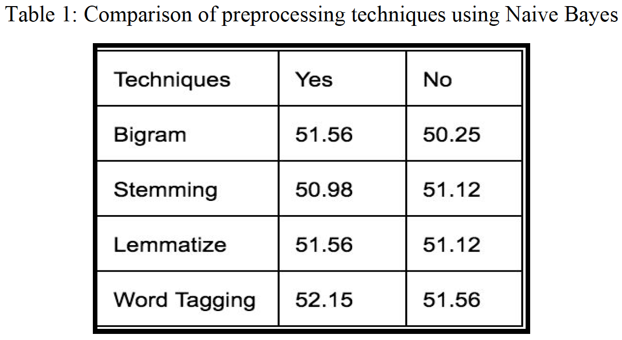
Based on table 1, which plots the accuracy of the Naive Bayes model, we observe that none of the preprocessing techniques significantly improves the performance of the classification. We also notice that Stemming, which reduces words to roots of words, isn’t as informative as Lemmatizing since the roots of words may not have been used in the actual articles. That’s why we need to be careful applying the different techniques that are commonly used for machine learning problems: the techniques might degrade instead improve the model performance if it’s not suited for our data. It’s also commonly known that bigram might degrade our classification as it increases our features size without adding more useful information. Table 1 shows that the combination of bigram, lemmatizing, and word tagging works the best. However, Table 1 also shows that the accuracy of most algorithms is very low, almost equivalent to random guessing. We think that this is due to the curse of dimensionality, since we have lots of features with only a sample size of 1254 and a feature size of 3455, worsening the sparseness of the data. Next, we want to investigate how the performance of text classification improves with increasing sample size.

Step 2: Generate labels for text classification

To perform any classification task, we need to have a labels for our data. Because we wanted to investigate how the news related to the stock movements, we decided that we should use some indicators of stock as the labels for the sentiment analysis model. One common binary stock indicator is comparing the stock returns with the return of S&P 500 index. This is a considerable assumption since the classification is assigned by aggregating the trades of everyone who reacts to the news, as well as the trades of other agents whose decisions are independent of what is in the news. So, to remedy this, we also did some experiments with another label involving the abnormal returns of a company.

Option 1: S&P 500 Comparison

We generate the stock return by computing the percentage of change in a company’s adjusted closing price within a one-day period. The return of the S&P 500 index is the average of stock returns for 500 standard companies. If the company’s return is above the S&P 500’s return, the label is 1, which signifies the company outperforms the market. On the other hand, the label is -1 to indicate that the company underperforms the market

Option 2: Abnormal Returns

Because “S&P500 comparison” label has many big assumptions, we try to experiment the sentiment model with another label which is abnormal return. Abnormal returns is the stock return of a company that is independent from the market movements. It’s the quantity that captures only the risk that is unique to the company’s stock. Abnormal Return is the difference between the actual return of a security and the expected return. Abnormal returns are sometimes triggered by "events." Events can include mergers, dividend announcements, company earning announcements, interest rate increases, lawsuits, etc.[Wikipedia]

Step 3: Compare performance of 2 Labels for text dataset

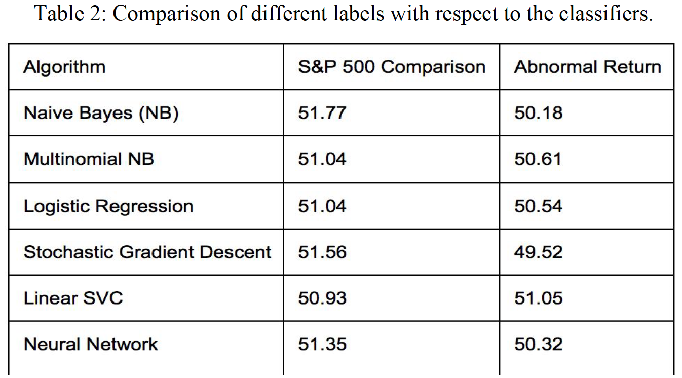
The financial news does respond slightly better on the S&P500 label as opposed to the abnormal return label. The difference is subtle, but this might be because the news is more likely to display the interaction of a company with the market rather than the sole well-beings of the company alone. The characteristics of the “S&P500 comparison” label indicate the performance of a company relative to the market, which more closely corresponds to the characteristics of the news data. Therefore, we decided to carry the sentiment scores generated by the text classification with the “S&P500 comparison” label to the stock classification.

Step 4: Experiment on Different Algorithms and Sample Size

Now that we’ve decided the best label to use for our sentiment analysis problem, we proceed to improve the performance of our classifiers by finding the optimal algorithm and sample size to find the best sentiment classifier.

We conducted experiments on 12 of the most common algorithms for text classification, and we picked the top 4 algorithms with the best trend of performance to plot the accuracy of these algorithms varying by sample size. Figure 1 shows that Multinomial Naïve Bayes and Neural Networks generally performs the best. Also, all algorithms get the highest accuracy with the sample size of approximately 1500 news events. Noise starts to appear after 1800 samples.

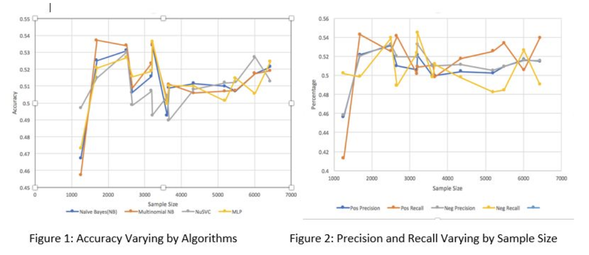
Positive recall is the percentage of positive news that is correctly classified, and positive precision is the probability that the file is classified correctly given that the file is labelled as positive. Figure 2 shows that the accuracy and precision on negative and positive news is generally equal. This means that most classifiers perform equally on both negative and positive files.

After the analysis, we used a sample size of 1800 to train our sentiment classifiers. To improve the quality of the sentiment scores generated by these classifiers, we created a voting system that includes the 10 best algorithms with tuned parameters that performs optimally with a sample size of 1800. We then fed each news event through each classifier, and the final score would be the percentage of the 10 best classifiers. For instance, if 85% of the classifiers classify a news event as negative, it means the sentiment score on that date for the given company is -0.85

These text classification experiments really reveal many weaknesses of the ‘Bag of Words’ approach. Even though it’s a well-known model for text classification with decent performance, being easy to compute and having some basic metric to extract the most descriptive terms in a document, this approach does not capture the position in text, semantics, and co-occurrences. Therefore, it is only useful as a lexical level feature. When it comes to financial news with many layers of complexity in features to describe a variety of topics, “Bag of Words” fails to give a decent result. Another reason for our bad results is that normally, text classification requires a very big sample size (more than 100,000 records) to overcome the noise normally inherent in the text data. If we look at figure 1, we can see that even though 1800 is the optimal sample size, we can see as the sample size get bigger, the accuracy slightly increases. We can thus expect that when the sample size is around 10 or 15 times of what we have right now, with the current increasing slope, it can hopefully reach a decent accuracy. Moreover, in the future, we could try applying some feature reduction using Information Gain to determine the most informative features for classification and only include those in our lexicon. This could help to reduce the sparseness of our feature sets.

3. Model 2: Stock Classification

Since we have a combination of 3 different data sources, so we think it would be a fun experiment to perform the classification model on different combination of data sources.

Dataset 1: Historical stock price

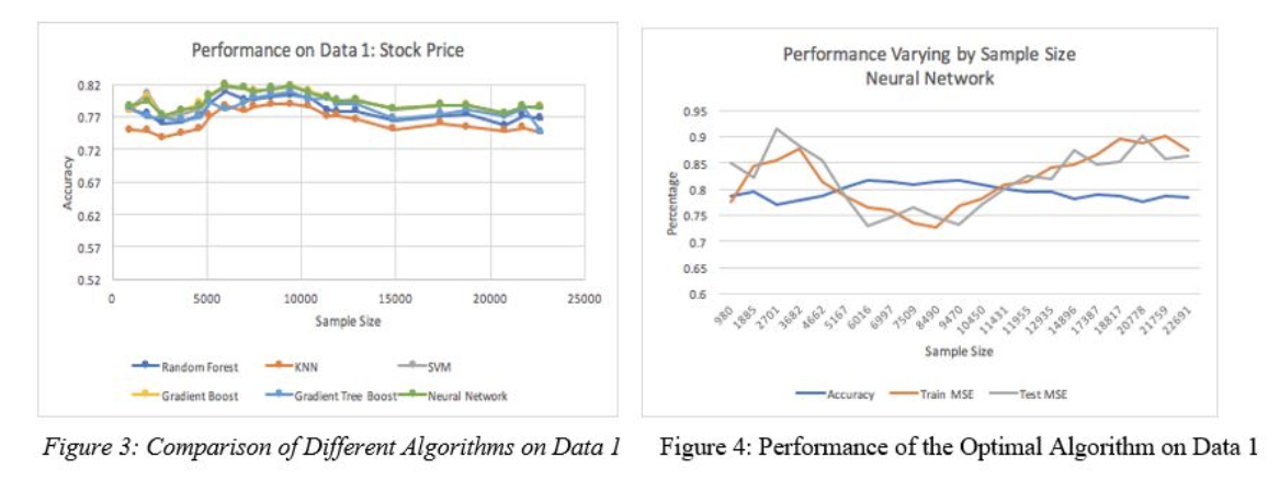
Figure 3 shows that accuracy is consistent as the sample size changes. There’s no significant differences in performance of different algorithms. Yet, Neural Network seems to perform the best in this case, so we proceed to investigate the training and testing MSE of the Neural Network. First, from theory, we expect that as the sample size increases, the testing MSE would decrease because the classifier can generalize the data better, while the training MSE increases as we introduce more noise. The intersection of training and testing MSE is the optimal sample size. However, figure 4 shows that for the first 3,000 samples, both training and testing MSE increase, and they decrease after 3,000 samples and increases again after 10,000 samples. This might be because in our process, we concatenate stock price of many companies and shuffle the samples, yet some of these companies in our data might not conform to the market trends or the common stock performance of other companies. That’s why we have a lot of noise in our data. However, with bigger sample sizes of perhaps 500 or so companies, our data might generalize these patterns better. Yet it’s too expensive for us to scrape news for more than 500 in a 6-year time frame, so we stuck with our 21 companies for this experiment.

Dataset 2: Historical stock price combined with fundamental Data

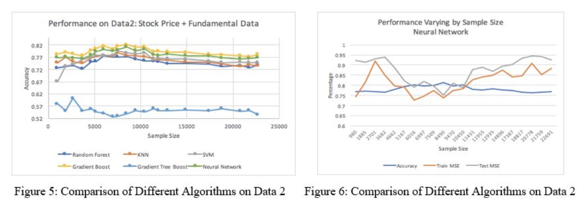
In figure 5, as we add extra fundamental data, we see that most of the classifiers perform similarly to dataset 1. The Quadratic Discriminant Analysis (QDA) performs noticeably the worst because QDA classifiers with quadratic decision boundaries are generated by fitting class conditional densities to the data using Bayes ‘rule. However, the fundamental data only changes around 24 times for the entire datasets due to being quarterly, so we’re dealing with many duplicate-values in our data, which is hard for Bayes Rule to generalize. Also, since different companies might have different features for fundamental data, merging these records together might leave many missing values. We did interpolate them based on time index, but it didn’t seem to improve the performance much. In a nutshell, the structure of dataset 2 doesn’t work well with the probability-based algorithm. Gradient Boosting performs the best because it uses a boosting method in which the last learner improves its performance by learning the previous learner. This process works well with the second dataset which has mixed data types of continuous, duplicate, and missing values. It’s hard for 1 algorithm to generalize all of these data types, so boosting, which combines multiple learners, optimizes performance in this case. Figure 6 shows that the training and testing MSE shows the same pattern as in dataset 1.

Dataset 3: Historical stock price, fundamental data and sentiment scores

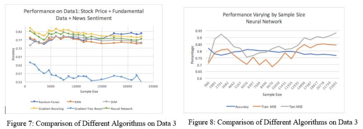Figures 7 and 8 show that by adding sentiment scores into the data, the accuracy patterns of dataset 3 is very similar to that of dataset 2, but the accuracy is slightly improved by around 2%. The Neural Network and the Gradient Boosting classifiers consistently perform well on 3 different combinations of data. Neural Network has its own feature transformation embedded within its algorithm, so it might help to improve the accuracy of our datasets 2 and 3 with more than 200 features. Gradient Boosting builds an additive model in a forward stage-wise fashion, which allows for the optimization of an arbitrary differentiable loss function.

Comparison of different data sources

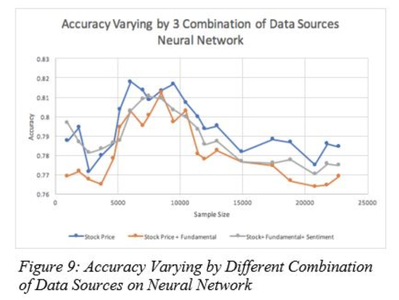
We can see that Neural Network consistently perform well on our prediction model. Therefore, we use this algorithm as the base model to compare the characteristics of the 3 different data sources. Figure 9 shows that contrast to our initial hypothesis that the additional fundamental data and sentiment scores would give us a better idea of the trends of the stock movements and accuracy in predicting the movement, it appears that using just the historical stock data performs the best in terms of accuracy. This might be because we added an extra 198 features into our dataset without increasing the sample size. Thus, we might not have enough data to converge these big sample sizes to a good result. We also notice that adding sentiment scores slightly increases the performance of classification approximately 2% to 3%. This is not a statistically significant improvement, but it’s most likely because the accuracies of the prior sentiment classifiers were only around 53%. With improvement on the text classifiers, we can expect to get a more significant impact of sentiment score on the stock classification. Moreover, we expect the sheer feature size might degrade the performance of stock classification on datasets 2 and 3. Therefore, we try some simple dimensionality transformation such as PCA on the dataset 3 to check whether the performance of our classifier would improve for future work.

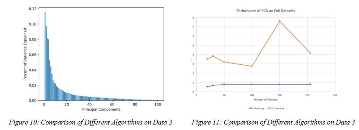
Figure 10 shows that 89% of variance is explained by the first 50 PCA components. However, figure 11 shows that PCA generally doesn’t help to improve the performance of the Neural Network algorithm, as after 50 components in PCA, the accuracy stays almost the same while PCA generally increases the training time. The end point on figure 11 is the accuracy and training time without PCA. It means that the transformation of our feature space to another dimension only worsens the performance. This might be because our data has many variance that are hard to capture.

Impacts of Different Sentiment Analysis Techniques on Stock Classification

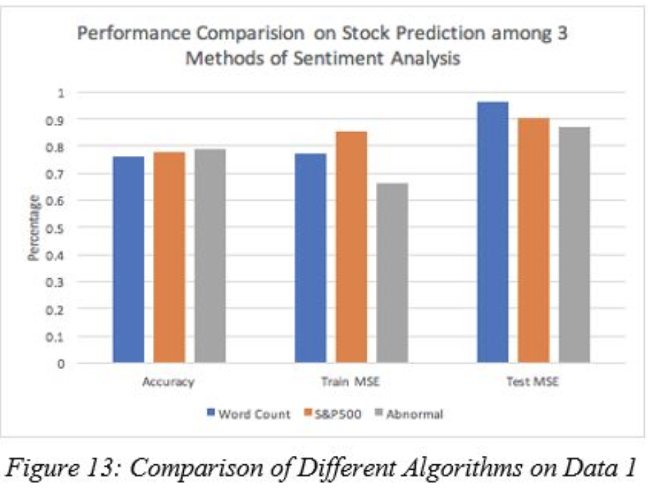
Initially, we did make an assumption that the sentiment score generated from the sentiment classification model using “S&P 500 Comparison” as a label would be the optimal additional features for our stock classification, yet the difference between the 2 labels were minor. We suspect that the ‘Bag of Words’ models actually performs better than other simpler model such as Word Count model. Word Count model is the simplest way to extract sentiment scores by counting the number of words that match the “Loughran McDonal” dictionary containing the 2000 most commonly used positive and negative words. Then we subtract the number of positive words from the number of negative words. We can observe on Figure 13 that the impact of sentiment scores generated by the ‘WordCount’ model is pretty close to the ones generated by the ‘Bag of Words’ model with 2 different labels. Moreover, it seems that unlike our prior belief, even though the accuracy of text classification with the ‘S&P500’ label is slightly higher than the one with ‘Abnormal Return’ label, the sentiment score generated by text classifier with the ‘Abnormal Return’ label is slightly better than the other two.

Comparison of stock classification labels

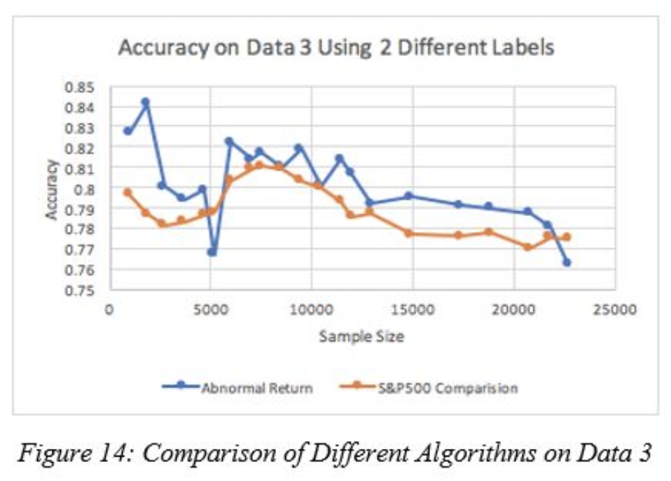Figure 14 reveals that the even though we are using the “S&P500” label as our target for most of the analysis in stock classification, it seems that our current data better predicts the ‘abnormal return’ than the comparison of company to the market. This might be because our data is mainly composed of features that reveal the characteristics of the company itself rather than the company performance compared to the market. More specifically, 198 fundamental features describe the characteristics of an individual company alone. Only the news sentiment scores and the stock prices are a few parameters that reflect the impact of market on the company stock performance.

Conclusion

Some interesting take-away facts from our project is that sentiment scores indeed slightly improve the performance of stock prediction. However, because we merge the stock on the same days that the news was published, it might not give us more informative decisions to buy the stock or not.

Moreover, it’s important that even though we get the best accuracy of approximately 81% with Neural Network model, does this model can really help us to make an informative decision on buying stock? When it comes to investment, what matters the most is the amount of returns. Classification would give us some relative ideas about the performance of the company compared to the market, but it doesn’t tell the whole story. We rather to make a lot of misclassification on the companies that have low return and make it up with a few right classifications on the companies that have high return. This, in turn, might give us a higher return in our portfolio than the one with higher accuracy. Therefore, one of the future work might be proceed to perform a regression problem to get an estimated return on stock.

Future Works

Insider Information

we should consider moving the time frame of the news 1 day before the stock prices is announced to check whether with some insider information would impact the performance more significantly.

Regression instead of Classification

Improve Sentiment Scores with Word Embedding

Instead of BoW, use Word Embedding or Topic Models for text classification